N170 Load and Visualize Data

This example demonstrates loading, organizing, and visualizing ERP response data from the visual P300 experiment.

Images of cats and dogs are shown in a rapid serial visual presentation (RSVP) stream.

The data used is the first subject and first session of the one of the eeg-notebooks P300 example datasets, recorded using the InteraXon MUSE EEG headset (2016 model). This session consists of six two-minute blocks of continuous recording.

We first use the fetch_datasets to obtain a list of filenames. If these files are not already present in the specified data directory, they will be quickly downloaded from the cloud.

After loading the data, we place it in an MNE Epochs object, and obtain the trial-averaged response.

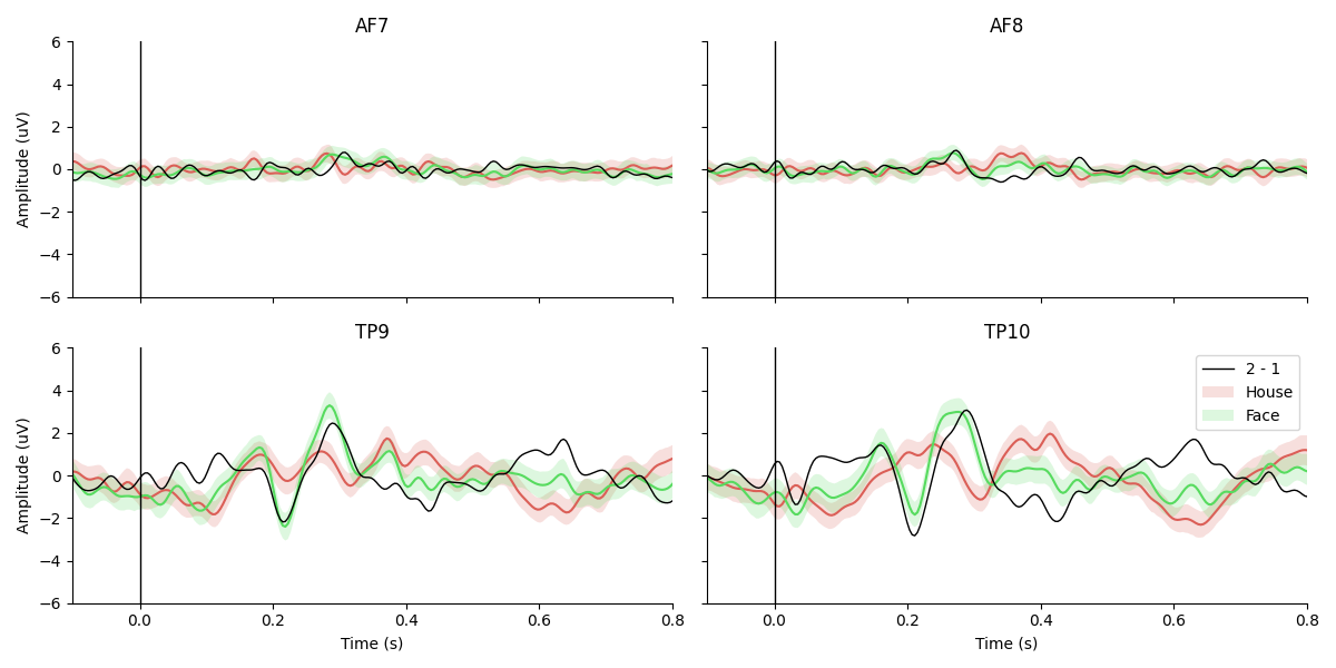
The final figure plotted at the end shows the P300 response ERP waveform.

Setup

# Some standard pythonic imports
import os
from collections import OrderedDict
import warnings
warnings.filterwarnings('ignore')

# MNE functions
from mne import Epochs,find_events

# EEG-Notebooks functions
from eegnb.analysis.utils import load_data,plot_conditions
from eegnb.datasets import fetch_dataset

# sphinx_gallery_thumbnail_number = 3

Load Data

We will use the eeg-notebooks N170 example dataset

Note that if you are running this locally, the following cell will download the example dataset, if you do not already have it.

eegnb_data_path = os.path.join(os.path.expanduser('~/'),'.eegnb', 'data')
n170_data_path = os.path.join(eegnb_data_path, 'visual-N170', 'eegnb_examples')

# If dataset hasn't been downloaded yet, download it
if not os.path.isdir(n170_data_path):
    fetch_dataset(data_dir=eegnb_data_path, experiment='visual-N170', site='eegnb_examples');

subject = 1
session = 1
raw = load_data(subject,session,
                experiment='visual-N170', site='eegnb_examples', device_name='muse2016',
                data_dir = eegnb_data_path)

Out:

['TP9', 'AF7', 'AF8', 'TP10', 'Right AUX', 'stim']
Creating RawArray with float64 data, n_channels=6, n_times=30720
    Range : 0 ... 30719 =      0.000 ...   119.996 secs
Ready.
['TP9', 'AF7', 'AF8', 'TP10', 'Right AUX', 'stim']
Creating RawArray with float64 data, n_channels=6, n_times=30732
    Range : 0 ... 30731 =      0.000 ...   120.043 secs
Ready.
['TP9', 'AF7', 'AF8', 'TP10', 'Right AUX', 'stim']
Creating RawArray with float64 data, n_channels=6, n_times=30732
    Range : 0 ... 30731 =      0.000 ...   120.043 secs
Ready.
['TP9', 'AF7', 'AF8', 'TP10', 'Right AUX', 'stim']
Creating RawArray with float64 data, n_channels=6, n_times=30732
    Range : 0 ... 30731 =      0.000 ...   120.043 secs
Ready.
['TP9', 'AF7', 'AF8', 'TP10', 'Right AUX', 'stim']
Creating RawArray with float64 data, n_channels=6, n_times=30732
    Range : 0 ... 30731 =      0.000 ...   120.043 secs
Ready.
['TP9', 'AF7', 'AF8', 'TP10', 'Right AUX', 'stim']
Creating RawArray with float64 data, n_channels=6, n_times=30732
    Range : 0 ... 30731 =      0.000 ...   120.043 secs
Ready.

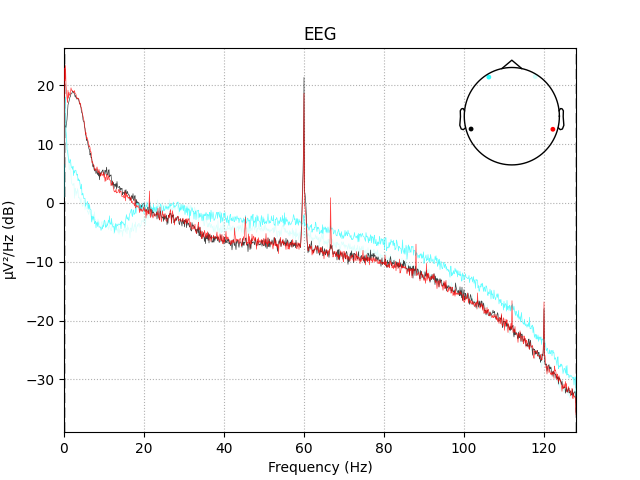
Visualize the power spectrum

raw.plot_psd()

Out:

Effective window size : 8.000 (s)
Generating pos outlines with sphere [0.    0.    0.    0.095] from [0.    0.    0.    0.095] for eeg
Generating coords using: [0.    0.    0.    0.095]

<Figure size 640x480 with 2 Axes>

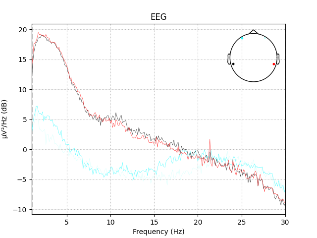
Filtering

raw.filter(1,30, method='iir')
raw.plot_psd(fmin=1, fmax=30);

Out:

Filtering raw data in 6 contiguous segments
Setting up band-pass filter from 1 - 30 Hz
Using filter length: 30732

IIR filter parameters
---------------------
Butterworth bandpass zero-phase (two-pass forward and reverse) non-causal filter:
- Filter order 16 (effective, after forward-backward)
- Cutoffs at 1.00, 30.00 Hz: -6.02, -6.02 dB

Effective window size : 8.000 (s)
Generating pos outlines with sphere [0.    0.    0.    0.095] from [0.    0.    0.    0.095] for eeg
Generating coords using: [0.    0.    0.    0.095]

<Figure size 640x480 with 2 Axes>

Epoching

# Create an array containing the timestamps and type of each stimulus (i.e. face or house)
events = find_events(raw)
event_id = {'House': 1, 'Face': 2}

# Create an MNE Epochs object representing all the epochs around stimulus presentation
epochs = Epochs(raw, events=events, event_id=event_id,
                tmin=-0.1, tmax=0.8, baseline=None,
                reject={'eeg': 75e-6}, preload=True,
                verbose=False, picks=[0,1,2,3])
print('sample drop %: ', (1 - len(epochs.events)/len(events)) * 100)
epochs

Out:

1174 events found
Event IDs: [1 2]
sample drop %:  4.003407155025551

<Epochs |  1127 events (all good), -0.101562 - 0.800781 sec, baseline off, ~8.0 MB, data loaded,
 'Face': 562
 'House': 565>

Epoch average

conditions = OrderedDict()
conditions['House'] = [1]
conditions['Face'] = [2]

fig, ax = plot_conditions(epochs, conditions=conditions,
                          ci=97.5, n_boot=1000, title='',
                          diff_waveform=(1, 2))